Sections 10.1-10.3 - Foundation
Why and how to carry out multiple linear regression analysis, and how to interpret its results
Motivation
There is a substantial difference in the average earnings of women and men in all countries. You want to understand more about the potential origins of that difference, focusing on employees with a graduate degree in your country. You have data on a large sample of employees with a graduate degree, with their earnings and some of their characteristics, such as age and the kind of graduate degree they have. Women and men differ in those characteristics, which may affect their earnings. How should you use this data to uncover gender difference that are not due to differences in those other characteristics? And can you use regression analysis to uncover patterns of associations between earnings and those other characteristics that may help understand the origins of gender differences in earnings?
You have analyzed your data on hotel prices in a particular city to find hotels that are underpriced relative to how close they are to the city center. But you have also uncovered differences in terms of other features of the hotels that measure quality and are related to price. How would you use this data to find hotels that are underpriced relative to all of their features? And how can you visualize the distribution of hotel prices relative to what price you would expect for their features in a way that helps identify underpriced hotels?
After understanding simple linear regression, we can turn to multiple linear regression, which has more than one explanatory variable. Multiple linear regression is the most used method to uncover patterns of associations between variables. There are multiple reasons to include more explanatory variables in a regression. We may be interested in uncovering patterns of association between y and other explanatory variables, which may help understand differences in terms of the x variable we are interested in most. Or, we may be interested in the effect of an x variable, but we want to compare observations that are different in x but similar in other variables. Finally, we may want to predict y, and we want to use more x variables to arrive at better predictions.
We discuss why and when we should estimate multiple regression, how to interpret its coefficients, and how to construct and interpret confidence intervals and test the coefficients. We discuss the relationship between multiple regression and simple regression. We explain that piecewise linear splines and polynomial regressions are technically multiple linear regressions without the same interpretation of the coefficients. We discuss how to include categorical explanatory variables as well as interactions that help uncover different slopes for groups. We include an informal discussions on how to decide what explanatory variables to include and in what functional form. Finally, we discuss why a typical multiple regression with observational data can get us closer to causal interpretation without fully uncovering it.
The first case study in this chapter, Understanding the gender difference in earnings, uses the cps-earnings data to illustrate the use of multiple regression to understand potential sources of gender differences in earnings. We also go back to our question on finding underpriced hotels relative to their location and quality in the case study Finding a good deal among hotels with multiple regression, using the hotels-vienna data, to illustrate the use of multiple regression in prediction and residual analysis.
Learning outcomes. After working through this chapter, you should be able to
🎯 Interactive Enhancements
This HTML version includes: - 🔗 Dashboard links to explore concepts visually - 💻 Codespace links to run analyses yourself - 🤖 AI practice tasks for personalized learning - 📊 Interactive figures and tables
There are three broad reasons to carry out multiple regression analysis instead of simple regression. The first is exploratory data analysis: we may want to uncover more patterns of association, typically to generate questions for subsequent analysis. The other two reasons are related to one of the two ultimate aims of data analysis: making a better prediction by explaining more of the variation, and getting closer to establishing cause and effect in observational data by comparing observations that are more comparable.
The first example of the introduction is about understanding the reasons of a difference. It’s a causal question of sorts: we are interested in what causes women to earn less than men. The second example is one of prediction: we want to capture average price related to hotel features that customers value in order to identify hotels that are inexpensive compared to what their price “should be.”
Prompt: “I’m studying the relationship between education and earnings. What are three variables I should ‘control for’ in a multiple regression, and why would omitting them bias my results?”
Multiple regression analysis uncovers average y as a function of more than one x variable: yE = f(x1, x2, ...). It can lead to better predictions of ŷ by considering more explanatory variables. It may improve the interpretation of slope coefficients by comparing observations that are different in terms of one of the x variables but similar in terms of all other x variables.
Multiple linear regression specifies a linear function of the explanatory variables for the average y. Let’s start with the simplest version with two explanatory variables:
yE = β0 + β1x1 + β2x2
This is the standard notation for a multiple regression: all coefficients are denoted by the Greek letter β, but they have subscripts. The intercept has subscript 0, the first explanatory variable has subscript 1, and the second explanatory variable has subscript 2.
Having another right-hand-side variable in the regression means that we take the value of that other variable into account when we compare observations. The slope coefficient on x1 shows the difference in average y across observations with different values of x1 but with the same value of x2. Symmetrically, the slope coefficient on x2 shows difference in average y across observations with different values of x2 but with the same value of x1. This way, multiple regression with two explanatory variables compares observations that are similar in one explanatory variable to see the differences related to the other explanatory variable.
The interpretation of the slope coefficients takes this into account. β1 shows how much larger y is on average for observations in the data with one unit larger value of x1 but the same value of x2. β2 shows how much larger y is on average for observations in the data with one unit larger value of x2 but with the same value of x1.
Multiple linear regression with two explanatory variables
yE = β0 + β1x1 + β2x2
Interpretation of the coefficients
Prompt: “I ran a regression: Price = 50 + 10×Bedrooms + 5×SquareFeet. How would I interpret the coefficient on Bedrooms? Write it in plain English as if explaining to a non-statistician.”
It is instructive to examine the difference in the slope coefficient of an explanatory variable x1 when it is the only variable on the right-hand-side of a regression compared to when another explanatory variable, x2, is included as well. In notation, the question is the difference between β in the simple linear regression
yE = α + βx1
and β1 in the multiple linear regression
yE = β0 + β1x1 + β2x2
For example, we may use time series data on sales and prices of the main product of our company, and regress month-to-month change in log quantity sold (y) on month-to-month change in log price (x1). Then β shows the average percentage change in sales when our price increases by one percent. For example, β̂ = −0.5 would show that sales tend to decrease by half of a percent when our price increases by one percent.
But we would like to know what happens to sales when we change our price but competitors don’t. The second regression has change in the log of the average price charged by our competitors (x2) next to x1. Here β1 would answer our question: average percentage change in our sales in months when we increase our price by one percent, but competitors don’t change their price. Suppose that in that regression, we estimate β̂1 = −3. That is, our sales tend to drop by 3 percent when we increase our price by 1 percent and our competitors don’t change their prices. Also suppose that the coefficient on x2 is positive, β̂2 = 3. That means that our sales tend to increase by 3 percent when our competitors increase their prices by 1 percent and our price doesn’t change.
As we’ll see, whether the answer to the two questions is the same will depend on whether x1 and x2 are related. To understand that relationship, let us introduce the regression of x2 on x1, called the x − x regression, where δ is the slope parameter:
x2E = γ + δx1
In our own price–competitor price example, δ would tell us how much the two prices tend to move together. In particular, it tells us about the average percentage change in competitor price in months when our own price increases by one percent. Let’s suppose that we estimate it to be δ̂ = 0.8: competitors tend to increase their price by 0.8 of a percent when our company increases its price by one percent. The two prices tend to move together, in the same direction.
To link the two original regressions, plug this x − x regression back in the multiple regression (this step is fine even though that may not be obvious; see Section 10.14):
yE = β0 + β1x1 + β2(γ + δx1) = β0 + β2γ + (β1 + β2δ)x1
Importantly, we find that with regards to x1, the slope coefficients in the simple (β) and multiple regression (β1) are different:
β − β1 = δβ2
The slope of x1 in a simple regression is different from its slope in the multiple regression, the difference being the product of its slope in the regression of x2 on x1 and the slope of x2 in the multiple regression. Or, put simply, the slope in simple regression is different from the slope in multiple regression by the slope in the x − x regression times the slope of the other x in the multiple regression.
This difference is called the omitted variable bias. If we are interested in the coefficient on x1 with x2 in the regression, too, it’s the second regression that we need, the first regression is an incorrect regression as it omits x2. Thus, the results from that first regression are biased, and the bias is caused by omitting x2. We will discuss omitted variables bias in detail when discussing causal effects in Chapter 21, Section 21.3.
In our sales–own price–competitors’ price example, we had that β̂ = −0.5 and β̂1 = −3, so that β̂ − β̂1 = −0.5 − (−3) = +2.5. In this case our simple regression gives a biased, overestimated slope on x1 compared to the multiple regression. Recall that we had δ̂ = 0.8 and β̂2 = 3. Their product is approximately 2.5 (2.4, but that difference is due to rounding). This overestimation is the result of two things: a positive association between the two price changes (δ) and a positive association between competitor price and our own sales (β2).
In general, the slope coefficient on x1 in the two regressions is different unless x1 and x2 are uncorrelated (δ = 0) or the coefficient on x2 is zero in the multiple regression (β2 = 0). The slope in the simple regression is larger if x2 and x1 are positively correlated and β2 is positive (or they are negatively correlated and β2 is negative).
The intuition is the following. In the simple regression yE = α + βx1, we compare observations that are different in x1 without considering whether they are different in x2. If x1 and x2 are uncorrelated this does not matter. In this case observations that are different in x1 are, on average, the same in x2, and, symmetrically, observations that are different in x2 are, on average, the same in x1. Thus the extra step we take with the multiple regression to compare observations that are different in x1 but similar in x2 does not matter here.
If, however, x1 and x2 are correlated, comparing observations with or without the same x2 value makes a difference. If they are positively correlated, observations with higher x2 tend to have higher x1. In the simple regression we ignore differences in x2 and compare observations with different values of x1. But higher x1 values mean higher x2 values, too. Corresponding differences in y may be due to differences in x1 but also due to differences in x2.
Key Takeaway on Omitted Variable Bias
When we omit an important variable from our regression: - The coefficient we estimate may be very different from the “true” effect - The direction and magnitude of bias depends on how the omitted variable relates to both y and the included x variables - Multiple regression helps us get closer to the right answer by including important covariates
Prompt: “Give me a real-world example (different from the textbook) where omitted variable bias would be a serious problem. Explain what the omitted variable is, what direction the bias would go, and why.”
Multiple linear regression
We continue investigating patterns in earnings, gender, and age. The data is the same cps-earnings data that we used earlier in Chapter 9, Section 9.2: it is a representative sample of all people of age 15 to 85 in the U.S.A. in 2014.
Compared to Chapter 9, Section 9.2, where we focused on a single occupation, we broaden the scope of our investigation here to all employees with a graduate degree – that is, a degree higher than a 4-year college degree: these include professional, master’s, and doctoral degrees.
We use data on people of age 24 to 65 (to reflect the typical working age of people with these kinds of graduate degrees). We excluded the self-employed (their earnings is difficult to measure) and included those who reported 20 hours or more as their usual weekly time worked. We have 18,241 observations.
The dependent variable is log hourly earnings ln w. Table 10.1 shows the results from three regressions. (1) is a simple regression of ln w on a binary female variable. (2) is a multiple regression that includes age as well, in a linear fashion. (3) is a simple regression with age as the dependent variable and the female binary variable.
# R Code to replicate Table 10.1
library(estimatr)
library(modelsummary)

# Load data
data <- read.csv("cps_earnings_grad.csv")

# Estimate three models
model1 <- lm_robust(lnearnings ~ female, data = data)
model2 <- lm_robust(lnearnings ~ female + age, data = data)
model3 <- lm_robust(age ~ female, data = data)

# Display results
modelsummary(list(model1, model2, model3),
             stars = c('***' = 0.01, '**' = 0.05, '*' = 0.1),
             gof_omit = "IC|Log|F|RMSE",
coef_rename = c("female" = "Female", "age" = "Age"))Table 10.1: Gender differences in earnings – log earnings and gender
| Variable | (1) ln w | (2) ln w | (3) age |
|---|---|---|---|
| female | -0.195*** | -0.185*** | -1.484*** |
| (0.008) | (0.008) | (0.159) | |
| age | 0.007*** | ||
| (0.000) | |||
| Constant | 3.514*** | 3.198*** | 44.630*** |
| (0.006) | (0.018) | (0.116) | |
| Observations | 18,241 | 18,241 | 18,241 |
| R-squared | 0.028 | 0.046 | 0.005 |
Note: All employees with a graduate degree. Robust standard error estimates in parentheses. *** p<0.01, ** p<0.05, * p<0.1
Source: cps-earnings dataset. 2014, U.S.A.
According to column (1), women in this sample earn 19.5 log points (around 21 percent) less than men, on average. Column (2) suggests that when we compare employees of the same age, women in this sample earn 18.5 log points (around 20 percent) less than men, on average. This is a slightly smaller gender difference than in column (1). While the log approximation is not perfect at these magnitudes, from now on, we will ignore the difference between log units and percent. For example, we will interpret a 0.195 coefficient as a 19.5 percent difference.
The estimated coefficients differ, and we know where the difference should come from: average difference in age. Let’s use the formula for the difference between the coefficient on female in the simple regression and in the multiple regression. Their difference is −0.195 − (−0.185) = −0.01. This should be equal to the product of the coefficient of female in the regression of age on female (our column (3)) and the coefficient on age in column (2): −1.48 × 0.007 ≈ −0.01. These two are indeed equal.
Intuitively, we can see that women of the same age have a slightly smaller earnings disadvantage in this data because they are somewhat younger, on average, and employees who are younger tend to earn less. Part of the earnings disadvantage of women is thus due to the fact that they are younger. This is a small part, though: around one percentage point of the 19.5% difference, which is a 5% share of the entire difference.
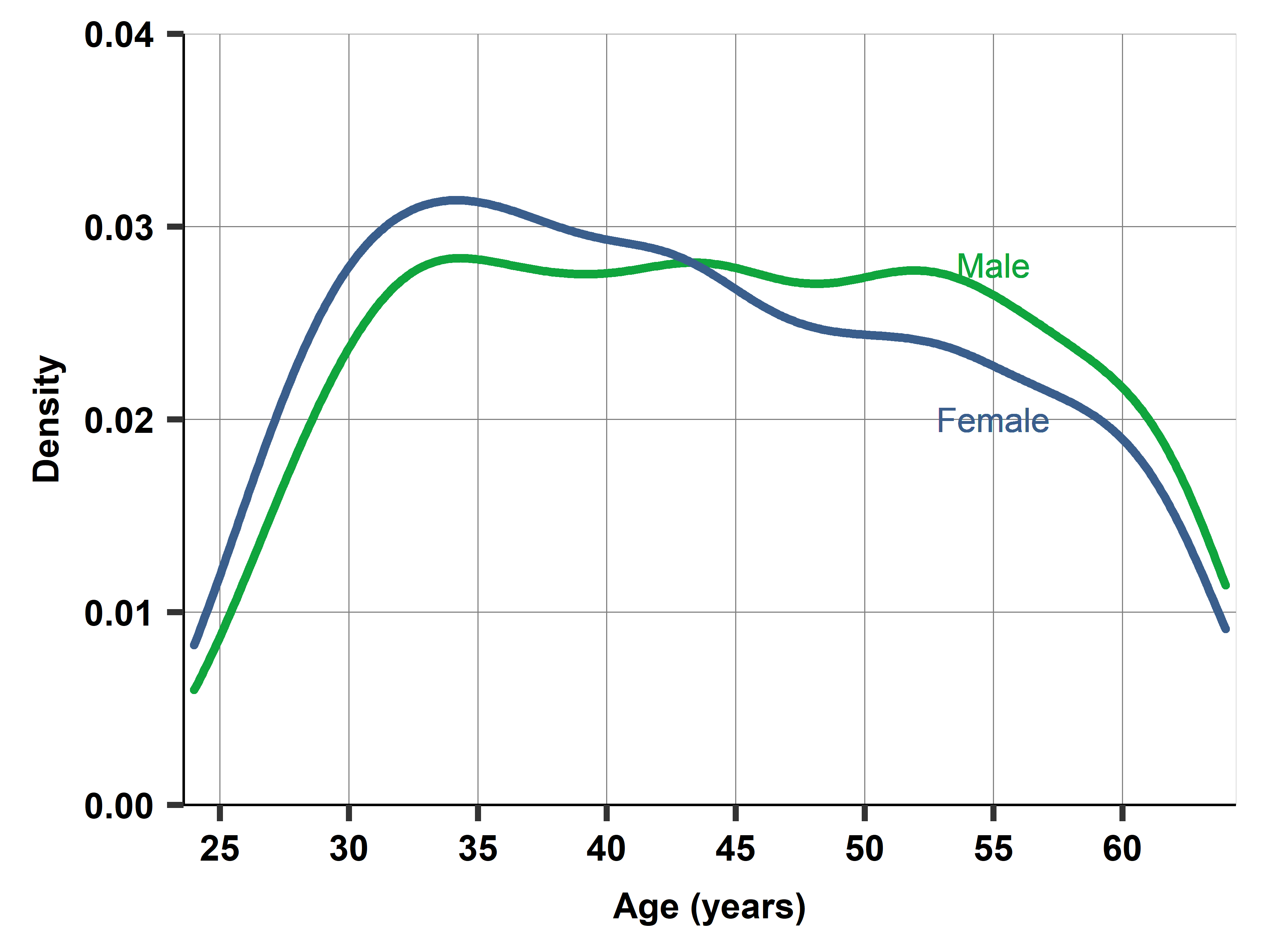
But why are women employees younger, on average, in the data? It’s because there are fewer female employees with graduate degrees over age 45 than below. Figure 10.1 shows two density plots overlaid: the age distributions of male and female employees with graduate degrees. There are relatively few below age 30. From age 30 and up, the age distribution is close to uniform for men. But not for women: the proportion of female employees with graduate degrees drops above age 45, and again above age 55.
# R Code to create Figure 10.1
library(ggplot2)
library(viridis)

ggplot(data, aes(x = age, fill = factor(female, labels = c("Male", "Female")))) +
  geom_density(alpha = 0.6) +
  scale_fill_manual(values = c("#20C997", "#D63384"), name = "") +
  labs(x = "Age (years)",
       y = "Density",
       title = "Age Distribution by Gender",
       subtitle = "Employees with Graduate Degrees") +
  theme_minimal(base_size = 12) +
  theme(legend.position = "top",
plot.title = element_text(face = "bold"))In principle, this could be due to two things: either there are fewer women with graduate degrees in the 45+ generation than among the younger ones, or fewer of them are employed (i.e., employed for 20 hours or more for pay, which is the criterion to be in our subsample). Further investigation reveals that it is the former: women are less likely to have a graduate degree if they were born before 1970 (those 45+ in 2014) in the U.S.A. The proportion of women working for pay for more than 20 hours is very similar among those below age 45 and above.
Look into conditional means by variables with our interactive dashboard. Adjust variables and watch the the graph change in real-time.
Prompt: “Looking at Table 10.1, explain why the coefficient on ‘female’ changes from -0.195 in column (1) to -0.185 in column (2). Use the omitted variable bias formula to verify this difference mathematically.”
🔗 Explore Further
Interactive Dashboard: Visualize multiple regression concepts and omitted variable bias
Open DashboardRun the Analysis: Replicate all regressions and create all figures yourself
Open in GitHub CodespaceDownload the Data: cps-earnings dataset
Get Data
This interactive HTML edition is a free companion to the full textbook. For the complete experience, please consider purchasing the book.
Buy from Cambridge University Press →