Sections 10.7-10.10 - Extensions & Interactions
Multiple explanatory variables, nonlinear patterns, categorical variables, and interactions
We spent a lot of time on multiple regression with two right-hand-side variables. That’s because that regression shows all the important differences between simple regression and multiple regression in intuitive ways. In practice, however, we rarely estimate regressions with exactly two right-hand-side variables. The number of right-hand-side variables in a multiple regression varies from case to case, but it’s typically more than two. In this section we describe multiple regressions with three or more right-hand-side variables. Their general form is
\[ y^E = \beta_0+\beta_1 x_1+\beta_2 x_2 +\beta_3 x_3+... \]
All of the results, language, and interpretations discussed so far carry forward to multiple linear regressions with three or more explanatory variables. Interpreting the slope of \(x_1\): on average, \(y\) is \(\beta_{1}\) units larger in the data for observations with one unit larger \(x_1\) but with the same value for all other \(x\) variables. The interpretation of the other slope coefficients is analogous. The language of multiple regression is the same, including the concepts of conditioning, controlling, omitted, or confounder variables.
The standard error of coefficients may be estimated by bootstrap or a formula. As always, the appropriate formula is the robust SE formula. But the simple formula contains the things that make even the robust SE larger or smaller. For any slope coefficient \(\hat{\beta}_k\) the simple SE formula is
\[ SE(\hat{\beta}_k)=\frac{Std[e]}{\sqrt{n}Std[x_k]\sqrt{1-R_{k}^2}} \]
Almost all is the same as with two right-hand-side variables. In particular, The SE is smaller, the smaller the standard deviation of the residuals (the better the fit of the regression), the larger the sample, and the larger the standard deviation of \(x_k\). The new-looking thing is \(R_{k}^2\). But that’s simply the generalization of \(R_{1}^2\) in the previous formula. It is the R-squared of the regression of \(x_k\) on all other \(x\) variables. The smaller that R-squared, the smaller the SE.
Equation:
\[ y^E = \beta_0+\beta_1 x_1+\beta_2 x_2 +\beta_3 x_3+... \]
Interpretation of \(\beta_{k}\) (slope of \(x_k\)):
Standard Error:
\[ SE(\hat{\beta}_k)=\frac{Std[e]}{\sqrt{n}Std[x_k]\sqrt{1-R_{k}^2}} \]
where \(e\) is the regression residual and \(R_{k}^2\) is the R-squared of the regression of \(x_k\) on all other \(x\) variables.
Prompt: “I’m estimating a regression with 5 explanatory variables. One of them (education) is highly correlated with the others. How will this affect the standard error of the education coefficient? Explain using the SE formula.”
In Chapter 8 we introduced piecewise linear splines, quadratics, and other polynomials to approximate a nonlinear \(y^E=f(x)\) regression.
From a substantive point of view, piecewise linear splines and polynomials of a single explanatory variable are not multiple regressions. They do not uncover differences with respect to one right-hand-side variable conditional on one or more other right-hand-side variables. Their slope coefficients cannot be interpreted as the coefficients of multiple regressions: it does not make sense to compare observations that have the same \(x\) but a different \(x^2\).
But such regressions are multiple linear regressions from a technical point of view. This means that the way their coefficients are calculated is the exact same way the coefficients of multiple linear regressions are calculated. Their standard errors are calculated the same way, too and so are their confidence intervals, test statistics, and p-values.
Testing hypotheses can be especially useful here, as it can help choose the functional form. With a piecewise linear spline, we can test whether the slopes are the same in adjacent line segments. If we can’t reject the null that they are the same, we may as well join them instead of having separate line segments. Testing hypotheses helps in choosing a polynomial, too. Here an additional complication is that the coefficients don’t have an easy interpretation in themselves. However, testing if all nonlinear coefficients are zero may help decide whether to include them at all.
However, testing hypotheses to decide whether to include a higher-order polynomial has its issues. Recall that a multiple linear regression requires that the right-hand-side variables are not perfectly collinear. In other words, they cannot be linear functions of each other. With a polynomial on the right-hand side, those variables are exact functions of each other: \(x^2\) is the square of \(x\). But they are not a linear function of each other, so, technically, they are not perfectly collinear. That’s why we can include both \(x\) and \(x^2\) and, if needed, its higher order terms, in a linear regression. While they are not perfectly collinear, explanatory variables in a polynomial are often highly correlated. That multicollinearity results in high standard errors, wide confidence intervals, and high p-values. As with all kinds of multicollinearity, there isn’t anything we can do about that once we have settled on a functional form.
Importantly, when thinking about functional form, we should always keep in mind the substantive focus of our analysis. As we emphasized in Chapter 8, Section 8.3, we should go back to that original focus when deciding whether we want to include a piecewise linear spline or a polynomial to approximate a nonlinear pattern. There we said that we want our regression to have a good approximation to a nonlinear pattern in \(x\) if our goal is prediction or analyzing residuals. We may not want that if all we care about is the average association between \(x\) and \(y\), except if that nonlinearity messes up the average association. This last point is a bit subtle, but usually means that we may want to transform variables to relative changes or take logs if the distribution of \(x\) or \(y\) is very skewed.
Here we have multiple \(x\) variables. Should we care about whether each is related to average \(y\) in a nonlinear fashion? The answer is the same as earlier: yes, if we want to do prediction or analyze residuals; no, if we care about average associations (except we may want to have transformed variables here, too). In addition, when we focus on a single average association (with, say, \(x_1\)) and all the other variables (\(x_2\), \(x_3\), …) are covariates to condition on, the only thing that matters is the coefficient on \(x_1\). Even if nonlinearities matter for \(x_2\) and \(x_3\) themselves, they only matter for us if they make a difference in the estimated coefficient on \(x_1\). Sometimes they do; very often they don’t.
Key Takeaway: When Does Functional Form Matter?
Functional form matters when: 1. Goal is prediction → Use best-fitting nonlinear patterns 2. Goal is residual analysis → Capture all patterns well 3. Nonlinearity affects the coefficient you care about
Functional form matters less when: 1. Goal is average association only 2. Nonlinearity in covariates doesn’t affect main coefficient 3. Focus is on direction not precise magnitude
Prompt: “I’m studying the effect of class size on test scores, controlling for school funding and teacher experience. Should I use a polynomial specification for the control variables? Explain your reasoning.”
Does nonlinear age pattern affect gender gap estimates?
This step in our case study illustrates the point we made in the previous section. The regressions in Table 10.2 enter age in linear ways. Using part of the same data, in Chapter 9, Section 9.2 we found that log earnings and age follow a nonlinear pattern. In particular, there we found that average log earnings are a positive and steep function of age for younger people, but the pattern becomes gradually flatter for the middle-aged and may become completely flat, or even negative, among older employees.
Should we worry about the non-linear age-earnings pattern when our question is the average earnings difference between men and women? We investigated the gender gap conditional on age. Table 10.2 shows the results for multiple ways of doing it. Column (1) shows the regression with the unconditional difference from Table 10.1, for reference. Column (2) enters age in linear form. Column (3) enters it as quadratic. Column (4) enters it as a fourth-order polynomial.
# R Code to replicate Table 10.2
library(estimatr)
library(modelsummary)

# Load data
data <- read.csv("cps_earnings_grad.csv")

# Model 1: Unconditional (for reference)
model1 <- lm_robust(lnearnings ~ female, data = data)

# Model 2: Linear age
model2 <- lm_robust(lnearnings ~ female + age, data = data)

# Model 3: Quadratic age
model3 <- lm_robust(lnearnings ~ female + age + I(age^2), data = data)

# Model 4: 4th-order polynomial
model4 <- lm_robust(lnearnings ~ female + age + I(age^2) + I(age^3) + I(age^4),
                    data = data)

# Display results
modelsummary(list(model1, model2, model3, model4),
             stars = c('***' = 0.01, '**' = 0.05, '*' = 0.1),
gof_omit = "IC|Log|F|RMSE")Table 10.2: Gender differences in earnings – log earnings and age, various functional forms
| Variable | (1) ln w | (2) ln w | (3) ln w | (4) ln w |
|---|---|---|---|---|
| female | -0.195*** | -0.185*** | -0.180*** | -0.180*** |
| (0.008) | (0.008) | (0.008) | (0.008) | |
| age | 0.007*** | -0.014 | 0.167** | |
| (0.000) | (0.010) | (0.075) | ||
| age² | 0.000 | -0.008** | ||
| (0.000) | (0.003) | |||
| age³ | 0.000** | |||
| (0.000) | ||||
| age⁴ | -0.000* | |||
| (0.000) | ||||
| Constant | 3.514*** | 3.198*** | 3.717*** | 2.152* |
| (0.006) | (0.018) | (0.202) | (1.113) | |
| Observations | 18,241 | 18,241 | 18,241 | 18,241 |
| R-squared | 0.028 | 0.046 | 0.048 | 0.051 |
Note: All employees with a graduate degree. Robust standard error estimates in parentheses. *** p<0.01, ** p<0.05, * p<0.1
Source: cps-earnings dataset. 2014 U.S.A.
The unconditional difference is -19.5%; the conditional difference is -18% according to column (2), and the same -18% according to columns (3) and (4). The various estimates of the conditional difference are the same up to two digits of rounding, and all of them are within each others’ confidence intervals. Thus, apparently, the functional form for age does not really matter if we are interested in the average gender gap.
At the same time, all coefficient estimates of the high order polynomials are statistically significant, meaning that the nonlinear pattern is very likely true in the population and not just a chance event in the particular dataset. The R-squared of the more complicated regressions are larger. These indicate that the complicated polynomial specifications are better at capturing the patterns. That would certainly matter if our goal was to predict earnings. But it does not matter for uncovering the gender difference in average earnings.
Key Insight
The nonlinear age-earnings relationship is real (statistically significant), but it doesn’t substantially affect our estimate of the gender wage gap. Why?
- The nonlinearity affects men and women similarly
- Age differences by gender are small
- Our focus is the gender coefficient, not perfect prediction
Bottom line: Functional form choices for control variables often don’t matter much when estimating treatment effects or group differences.
Prompt: “Looking at Table 10.2, explain why the R-squared increases from column (2) to column (4), but the gender coefficient stays essentially the same. What does this tell us about when functional form matters?”
A great advantage of multiple linear regression is that it can deal with binary and other qualitative explanatory variables (also called categories, factor variables), together with quantitative variables, on the right-hand-side.
To include such variables in the regression, we need to have them as binary, zero-one variables – also called dummy variables in the regression context. That’s straightforward for variables that are binary to begin with: assign values zero and one (as we did with \(female\) in the case study). We need to transform qualitative variables into binary ones, too, each denoting whether the observation belongs to that category (one) or not (zero). Then we need to include all those binary variables in the regression. Well, all except one.
We should select one binary variable denoting one category as a reference category, or reference group – also known as the “left-out category.” Then we have to include the binary variables for all other categories but not the reference category. That way the slope coefficient of a binary variable created from a qualitative variable shows the difference between observations in the category captured by the binary variable and the reference category. If we condition on other explanatory variables, too, the interpretation changes in the usual way: we compare observations that are similar in those other explanatory variables.
As an example, suppose that \(x\) is a categorical variable measuring the level of education with three values \(x=\{low, medium, high\}\). We need to create binary variables and include two of the three in the regression. Let the binary variable \(x_{med}\) denote if \(x=medium\), and let the binary \(x_{high}\) variable denote if \(x = high\). Include \(x_{med}\) and \(x_{high}\) in the regression. The third potential variable for \(x=low\) is not included. It is the reference category.
\[ y^E = \beta_0 + \beta_1 x_{med} + \beta_2 x_{high} \]
Let us start with the constant, \(\beta_0\); this shows average \(y\) in the reference category. Here, \(\beta_0\) is average \(y\) when both \(x_{med}=0\) and \(x_{high}=0\): this is when \(x=low\).
\(\beta_1\) is the difference in average \(y\) between observations that are different in \(x_{med}\) but the same in \(x_{high}\). Thus \(\beta_1\) shows the difference of average \(y\) between observations with \(x=medium\) and \(x=low\), the reference category. Similarly, \(\beta_2\) shows the difference of average \(y\) between observations with \(x=high\) and \(x=low\), the reference category.
Which category to choose for the reference? In principle that should not matter: choose a category and all others are compared to that, but we can easily compute other comparisons from those. For example, the difference in \(y^E\) between observations with \(x=high\) and \(x=medium\) in the example above is simply \(\beta_2 - \beta_1\) (both coefficients compare to \(x=low\), and that drops out of their difference). But the choice may matter for practical purposes. Two guiding principles may help this choice, one substantive, one statistical. The substantive guide is simple: we should choose the category to which we want to compare the rest. Examples include the home country, the capital city, the lowest or highest value group. The statistical guide is to choose a category with a large number of observations. That is relevant when we want to infer differences from the data for the population, or general pattern, it represents. If the reference category has very few observations, the coefficients that compare to it will have large standard errors, wide confidence intervals, and large p-values.
Example: Education with 3 levels (Low, Medium, High) * Create: \(x_{med}\) (=1 if Medium), \(x_{high}\) (=1 if High) * Leave out: Low (reference category) * Regression: \(y^E = \beta_0 + \beta_1 x_{med} + \beta_2 x_{high}\) * Interpretation: - \(\beta_0\) = Average \(y\) for Low education - \(\beta_1\) = Difference: Medium - Low - \(\beta_2\) = Difference: High - Low - \(\beta_2 - \beta_1\) = Difference: High - Medium
Prompt: “I have a categorical variable ‘region’ with 5 regions: North, South, East, West, Central. I want to include this in a regression. Show me how to set it up as dummy variables, explain which category to choose as reference, and interpret one coefficient.”
How do different graduate degrees relate to earnings?
Let’s use our case study to illustrate qualitative variables as we examine earnings differences by categories of educational degree. Recall that our data contains employees with graduate degrees. The dataset differentiates three such degrees: master’s (including graduate teaching degrees, MAs, MScs, MBAs etc.), professional (including MDs), and PhDs.
Table 10.3 shows the results from three regressions. As a starting point, column (1) repeats the results of the simple regression with \(female\) on the right-hand-side. Column (2) includes two education categories \(ed\_Profess\) and \(ed\_PhD\); Column (3) includes another set of education categories, \(ed\_Profess\) and \(ed\_MA\). The reference category is MA degree in column (2) and PhD in column (3).
# R Code to replicate Table 10.3
library(estimatr)
library(modelsummary)

# Load data
data <- read.csv("cps_earnings_grad.csv")

# Ensure education is a factor with MA as reference
data$education <- factor(data$grad_degree,
                        levels = c("MA", "Professional", "PhD"))

# Model 1: Baseline (gender only)
model1 <- lm_robust(lnearnings ~ female, data = data)

# Model 2: Gender + education (MA reference)
model2 <- lm_robust(lnearnings ~ female + education, data = data)

# Model 3: Gender + education (PhD reference)
data$education_phd_ref <- relevel(data$education, ref = "PhD")
model3 <- lm_robust(lnearnings ~ female + education_phd_ref, data = data)

# Display results
modelsummary(list(model1, model2, model3),
             stars = c('***' = 0.01, '**' = 0.05, '*' = 0.1),
gof_omit = "IC|Log|F|RMSE")Table 10.3: Gender differences in earnings – log earnings, gender and education
| Variable | (1) ln w | (2) ln w | (3) ln w |
|---|---|---|---|
| female | -0.195*** | -0.182*** | -0.182*** |
| (0.008) | (0.008) | (0.008) | |
| ed_Profess | 0.134*** | 0.002 | |
| (0.012) | (0.012) | ||
| ed_PhD | 0.136*** | ||
| (0.011) | |||
| ed_MA | -0.136*** | ||
| (0.011) | |||
| Constant | 3.514*** | 3.434*** | 3.570*** |
| (0.006) | (0.008) | (0.010) | |
| Observations | 18,241 | 18,241 | 18,241 |
| R-squared | 0.028 | 0.046 | 0.046 |
Note: The data includes employees with a graduate degree. MA, Professional and PhD are three categories of graduate degree. Column (2): MA is the reference category. Column (3): PhD is the reference category. Robust standard error estimates in parentheses. *** p<0.01, ** p<0.05, * p<0.1
Source: cps-earnings data. U.S.A., 2014.
The coefficients in column (2) of Table 10.3 show that comparing employees of the same gender, those with a professional degree earn, on average, 13.4% more than employees with an MA degree, and those with a PhD degree earn, on average, 13.6% more than employees with an MA degree. The coefficients in column (3) show that, among employees of the same gender, those with an MA degree earn, on average, 13.6% less than those with a PhD degree, and those with a professional degree earn about the same on average as those with a PhD degree. These differences are consistent with each other.
This is a large dataset so confidence intervals are rather narrow whichever group we choose as a reference category. Note that the coefficient on \(female\) is smaller, \(-0.182\), when education is included in the regression. This suggests that part of the gender difference is due to the fact that women are somewhat more likely to be in the lower-earner MA group than in the higher-earner professional or PhD groups. But only a small part. We shall return to this finding later when we try to understand the causes of gender differences in earnings.
Practical Tip: Choosing Reference Categories
Good reference categories: 1. Natural baseline (e.g., lowest education level) 2. Largest group (more observations = smaller SE) 3. Group you want to compare all others to 4. Control group in experiments
Computing other comparisons: - From column (2): Professional vs PhD = \(0.134 - 0.136 = -0.002\) (essentially the same) - This matches the Professional coefficient in column (3): \(0.002\)
Including binary variables for various categories of a qualitative variable uncover average differences in \(y\). But sometimes we want to know something more: whether and how much the slope with respect to a third variable differs by those categories. Multiple linear regression can uncover that too, with appropriate definition of the variables.
More generally, we can use the method of linear regression analysis to uncover how association between \(y\) and \(x\) varies by values of a third variable \(z\). Such variation is called an interaction, as it shows how \(x\) and \(z\) interact in shaping average \(y\). In medicine, when estimating the effect of \(x\) on \(y\), if that effect varies by a third variable \(z\), that \(z\) is called a moderator variable. Examples include whether malnutrition, immune deficiency, or smoking can decrease the effect of a drug to treat an illness. Non-medical examples of interactions include whether and how the effect of monetary policy differs by the openness of a country, or whether and how the way customer ratings are related to hotel prices differs by hotel stars.
Multiple regression offers the possibility to uncover such differences in patterns. For the simplest case, consider a regression with two explanatory variables: \(x_1\) is quantitative; \(x_2\) is binary. We wonder if the relationship between average \(y\) and \(x_1\) is different for observations with \(x_2=1\) than for \(x_2=0\). How shall we uncover that difference?
A multiple regression that includes \(x_1\) and \(x_2\) estimates two parallel lines for the \(y\) – \(x_1\) pattern: one for those with \(x_2=0\) and one for those with \(x_2=1\).
\[ y^E = \beta_0+\beta_1 x_1+\beta_2 x_2 \]
The slope of \(x_1\) is \(\beta_1\) and is the same in this regression for observations in the \(x_2=0\) group and observations in the \(x_2=1\) group. \(\beta_2\) shows the average difference in \(y\) between observations that are different in \(x_2\) but have the same \(x_1\). Since the slope of \(x_1\) is the same for the two \(x_2\) groups, this \(\beta_2\) difference is the same across the range of \(x_1\). This regression does not allow for the slope in \(x_1\) to be different for the two groups. Thus, this regression cannot uncover whether the \(y\) – \(x_1\) pattern differs in the two groups.
Denote the expected \(y\) conditional on \(x_1\) in the \(x_2=0\) group as \(y^E_0\), and denote the expected \(y\) conditional on \(x_1\) in the \(x_2=1\) group as \(y^E_1\). Then, the regression above implies that the intercept is different (higher by \(\beta_2\) in the \(x_2=1\) group) but the slopes are the same:
First group, \(x_2=0\): \[ y^E_0 = \beta_0 + \beta_1 x_1 \]
Second group, \(x_2=1\): \[ y^E_1 = \beta_0 + \beta_2 \times 1 + \beta_1 x_1 \]
If we want to allow for different slopes in the two \(x_2\) groups, we have to do something different. That difference is including the interaction term. An interaction term is a new variable that is created from two other variables, by multiplying one by the other. In our case:
\[ y^E = \beta_0+\beta_1 x_1+\beta_2 x_2 + \beta_3 x_1 x_2 \]
Not only the intercepts are different; the slopes are different, too.
First group, \(x_2=0\): \[ y^E_0 = \beta_0 + \beta_1 x_1 \]
Second group, \(x_2=1\): \[ y^E_1 = \beta_0 + \beta_2 + (\beta_1 + \beta_3) x_1 \]
It turns out that the coefficients of this regression can be related to the coefficients of two simple regressions of \(y\) on \(x_1\), estimated separately in the two \(x_2\) groups.
Separate regressions: \[ \begin{aligned} y^E_0 &= \gamma_0+\gamma_1 x_1 \\ y^E_1 &= \gamma_2+\gamma_3 x_1 \end{aligned} \]
What we have is \(\gamma_0=\beta_0\); \(\gamma_1=\beta_1\) ; \(\gamma_2=\beta_0+\beta_2\); and \(\gamma_3=\beta_1+\beta_3\);
In other words, the separate regressions in the two groups and the regression that pools observations but includes an interaction term yield exactly the same coefficient estimates. The coefficients of the separate regressions are easier to interpret. But the pooled regression with interaction allows for a direct test of whether the slopes are the same. \(H_0: \beta_3 = 0\) is the null hypothesis for that test; thus the simple t-test answers this question.
We can mix these tools to build ever more complicated multiple regressions. Binary variables can be interacted with other binary variables. Binary variables created from qualitative explanatory variables with multiple categories can all be interacted with other variables. Piecewise linear splines or polynomials may be interacted with binary variables. More than two variables may be interacted as well. Furthermore, quantitative variables can also be interacted with each other, although the interpretation of such interactions is more complicated.
General form: \[ y^E = \beta_0 + \beta_1 x_1 + \beta_2 x_2 + \beta_3 x_1 x_2 \]
Interpretation: * \(\beta_1\) shows average differences in \(y\) corresponding to a one-unit difference in \(x_1\) when \(x_2=0\). * \(\beta_2\) shows average differences in \(y\) corresponding to a one-unit difference in \(x_2\) when \(x_1=0\). * \(\beta_3\) is the coefficient on the interaction term. It shows the additional average differences in \(y\) corresponding to a one-unit difference in \(x_1\) when \(x_2\) is one unit larger, too. (It’s symmetrical in \(x_1\) and \(x_2\).)
When one variable is binary (\(x_2=0\) or \(1\)): * \(\beta_1\) shows average differences in \(y\) per unit of \(x_1\) when \(x_2=0\) * \(\beta_1 + \beta_3\) shows average differences in \(y\) per unit of \(x_1\) when \(x_2=1\) * Equivalent to running separate regressions for each group
Testing for different slopes: * \(H_0: \beta_3 = 0\) tests whether slopes are the same * Reject → slopes differ by group * Fail to reject → parallel lines okay
Prompt: “Explain interaction terms using this example: I’m studying how study hours affect test scores, and I suspect the effect might be different for students who attend tutoring vs those who don’t. Write out the regression equation with an interaction term and interpret each coefficient.”
Does the gender wage gap vary with age?
We turn to illustrating the use of interactions as we consider the question of whether the patterns with age are similar or different for men versus women. As we discussed, we can investigate this in two ways that should lead to the same result: estimating regressions separately for men and women and estimating a regression that includes age interacted with gender. This regression model with an interaction is:
\[ (\ln w)^E = \beta_0 + \beta_1 \times age + \beta_2 \times female + \beta_3 \times age \times female \]
Table 10.4 shows the results with age entered in a linear fashion. Column (1) shows the results for women, column (2) for men, column (3) for women and men pooled, with interactions. To have a better sense of the differences, which are often small, the table shows coefficients up to three digits.
# R Code to replicate Table 10.4
library(estimatr)
library(modelsummary)

# Load data
data <- read.csv("cps_earnings_grad.csv")

# Model 1: Women only
model1 <- lm_robust(lnearnings ~ age, data = subset(data, female == 1))

# Model 2: Men only
model2 <- lm_robust(lnearnings ~ age, data = subset(data, female == 0))

# Model 3: Pooled with interaction
model3 <- lm_robust(lnearnings ~ age + female + age:female, data = data)

# Display results
modelsummary(list(model1, model2, model3),
             stars = c('***' = 0.01, '**' = 0.05, '*' = 0.1),
             gof_omit = "IC|Log|F|RMSE",
fmt = 3) # Show 3 decimal placesTable 10.4: Gender differences in earnings – log earnings, gender, age, and their interaction
| Variable | (1) Women | (2) Men | (3) Pooled |
|---|---|---|---|
| age | 0.006*** | 0.009*** | 0.009*** |
| (0.001) | (0.001) | (0.001) | |
| female | -0.036 | ||
| (0.042) | |||
| age × female | -0.003*** | ||
| (0.001) | |||
| Constant | 3.081*** | 3.117*** | 3.117*** |
| (0.030) | (0.023) | (0.023) | |
| Observations | 7,874 | 10,367 | 18,241 |
| R-squared | 0.004 | 0.012 | 0.032 |
Note: Employees with a graduate degree. Column (1) is women only; column (2) is men only; column (3) includes all employees. Robust standard error estimates in parentheses. *** p<0.01, ** p<0.05, * p<0.1
Source: cps-earnings data. U.S.A., 2014.
According to column (1) of Table 10.4, women who are one year older earn 0.6 percent more, on average. According to column (2), men who are one year older earn 0.9 percent more, on average. Column (3) repeats the age coefficient for men. Then it shows that the slope of the log earnings – age pattern is, on average, 0.003 less positive for women, meaning that the earnings advantage of women who are one year older is 0.3 percentage points smaller than the earnings advantage of men who are one year older.
The advantage of the pooled regression, is its ability to allow for direct inference about gender differences. The 95% CI of the gender difference in the average pattern of ln wages and age is [-0.005,-0.001]. Among employees with post-graduate degree in the U.S.A. in 2014, the wage difference corresponding to a one year difference in age was 0.1 to 0.5 percentage points less positive for women than for men. This confidence interval does not include zero. Accordingly, the t-test of whether the difference is zero rejects its null at the 5% level, suggesting that we can safely consider the difference as real in the population (as opposed to a chance event in the particular dataset); we are less than 5% likely to make a mistake by doing so.
The coefficient on the \(female\) variable in the pooled regression is \(-0.036\). This is equal to the difference of the two regression constants: \(3.081\) for women and \(3.117\) for men. Those regression constants do not have a clear interpretation here (average log earnings when age is zero are practically meaningless). Their difference, which is actually the coefficient on \(female\) in the pooled regression, shows the average gender difference between employees with zero age. Similarly to the constants in the separate regressions, the coefficient is meaningless for any substantive purpose. Nevertheless, the regression needs it to have an intercept with the \(\ln w\) axis.
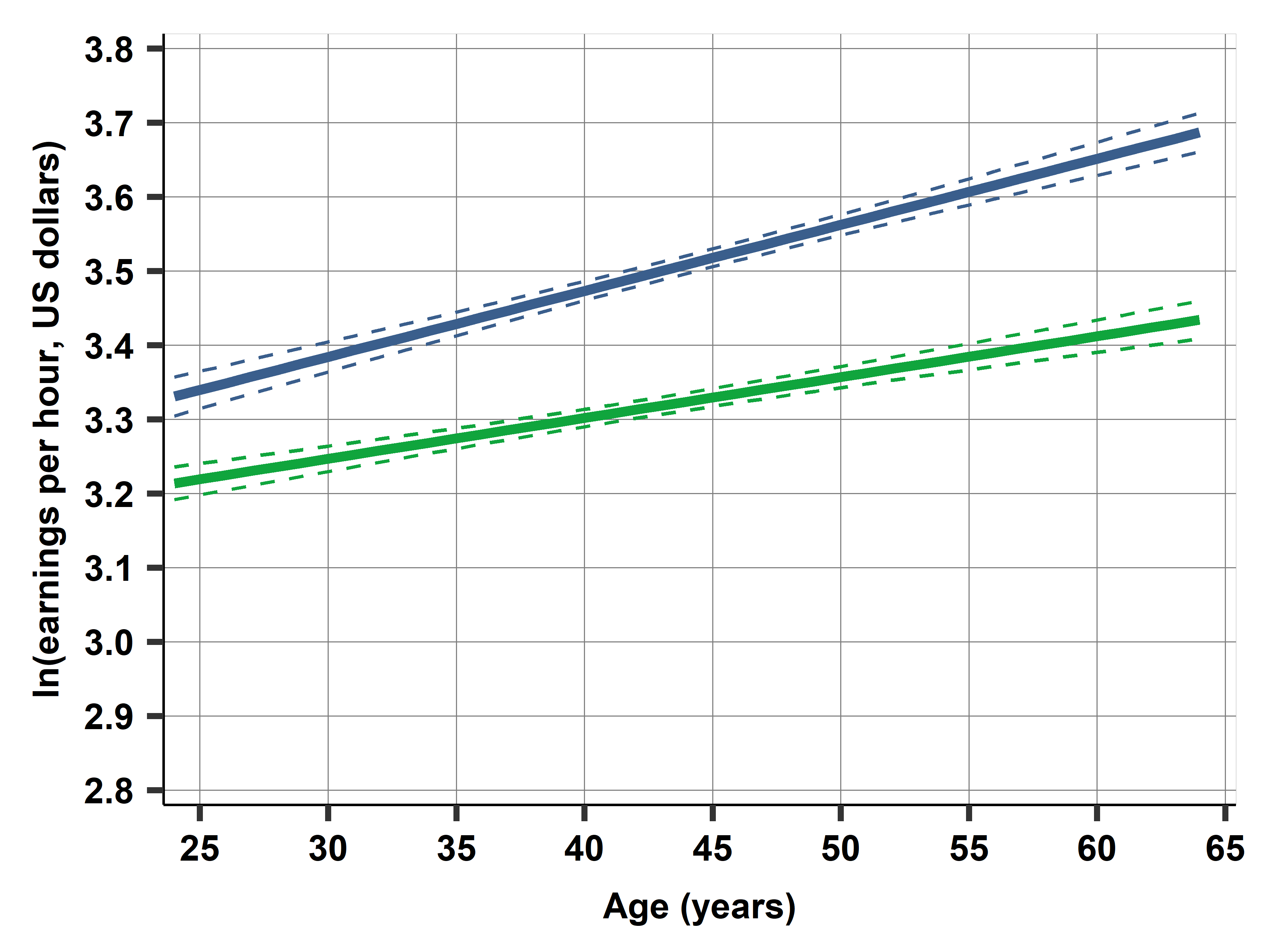
Taking the coefficients on \(female\), \(age\), and \(female \times age\) together, the regression allows us to calculate the average gender difference by age. This exercise takes the linear functional form seriously, an assumption we know is false. We shall repeat this exercise with a better approximation of the nonlinear patterns. For now, let’s stick to the linear specification, for educational purposes.
The youngest people in our sample are 25 years old. Starting with the separate regressions, the predicted log wage for women of age 25 is \(3.081 + 25 \times 0.006 \approx 3.231\). For men, \(3.117 + 25 \times 0.009 \approx 3.342\). The difference is \(-0.11\). We get the same number from the pooled regression: the gender difference at age 25 should be the gender difference at age zero implied by the coefficient on \(female\) plus 25 times the difference in the slope by age, the coefficient on the interaction term \(female \times age\): \(-0.036 + 25 \times -0.003 \approx -0.11\). Carrying out the same calculations for age 45 yields a difference of \(-0.17\). These results imply that the gender difference in average earnings is wider for older ages.
Figure 10.2a shows the relationship graphically. It includes two lines with a growing gap: earnings difference is higher for older age. Remember, our regression can capture this growing gap because it includes the interaction. Without the interaction, we would not be able to see this, as that specification would force two parallel lines at constant distance.
However, we know that the pattern on age and (log) earnings is not linear. Our earlier results indicate that a fourth-order polynomial is a better approximation to that pattern. To explore whether the shapes of the age-earnings profiles are different between women and men, we re-estimated the regression with age in a fourth-order polynomial interacted with gender:
\[ \begin{aligned} (\ln w)^E = &\beta_0 + \beta_1 age + \beta_2 age^2 + \beta_3 age^3 + \beta_4 age^4 + \beta_5 female \\ &+ \beta_6 female \times age + \beta_7 female \times age^2 \\ &+ \beta_8 female \times age^3 + \beta_9 female \times age^4 \end{aligned} \]
This is a complicated regression with coefficients that are practically impossible to interpret. We don’t show the coefficient estimates here. Instead we visualize the results. The graph in Figure 10.2b shows the predicted pattern (the regression curves) for women and men, together with the confidence intervals of the regression lines (curves here), as introduced in Chapter 9, Section 9.4.
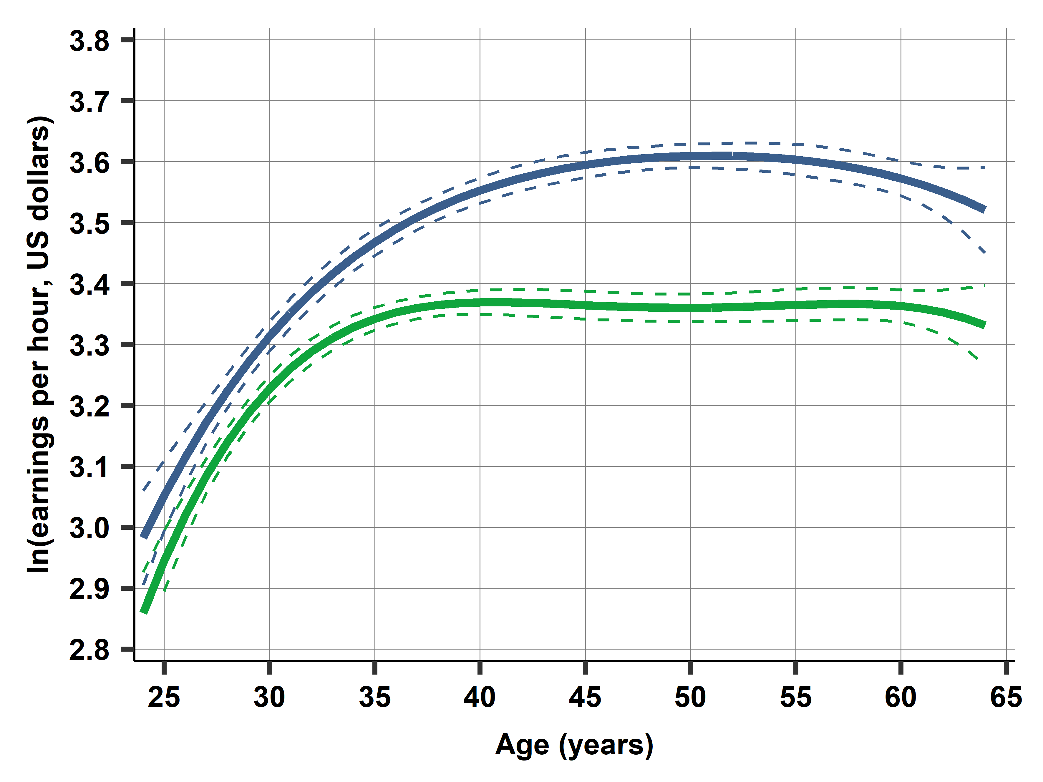
Figure 10.2b suggests that the average earnings difference is a little less than 10% between ages 25 and 30, increases to around 15% by age 40, and reaches 22% by age 50, from where it decreases slightly to age 60 and more by age 65. These differences are likely similar in the population represented by the data as the confidence intervals around the regression curves are rather narrow, except at the two ends.
These results are very informative. Many factors may cause women with a graduate degree to earn less than men. Some of those factors are present at young age, but either they are more important in middle age, or additional factors start playing a role by then.
Key Findings from Case Study A5
- The gender wage gap grows with age (from ~10% at age 25 to ~22% at age 50)
- The interaction is statistically significant (p < 0.01)
- This pattern is robust to different functional forms (linear vs polynomial)
- Policy implications: The growing gap suggests factors that accumulate over careers (promotion barriers, family responsibilities, discrimination)
What we can’t determine from this analysis: - Whether this is cohort effect vs age effect - Exact mechanisms causing the growing gap - Causal vs correlational interpretation
Prompt: “Looking at Figure 10.2b, explain why the confidence intervals are wider at the ends (ages 25 and 65) compared to the middle ages. What does this tell us about the reliability of our estimates?”
In this section we covered:
Next: In the final section, we’ll discuss how multiple regression relates to causal analysis and prediction.
🔗 Explore Further
Interactive Dashboard: Visualize interactions and categorical variables
Open DashboardRun the Analysis: Replicate all regressions yourself
Open in GitHub CodespaceDownload the Data: cps-earnings dataset
Get Data