Part I: DATA EXPLORATION

PART I: DATA EXPLORATION

CH01A Finding a good deal among hotels: data collection

Vienna, Austria is a popular tourist destination for business and leisure. From the hundreds of places that offer accommodation, we want to pick a hotel that is underpriced relative to its location and quality for a weekday in November 2017. Can we use data to help this decision? What kind of data would we need, and how could we get it?

This case study illustrates how to collect appropriate data from the web on multiple offers. It describes what we want from such data and what data source we would need. The data is collected by web scraping, and it results in a single data table. The case study discusses the data quality from the perspective of the question to answer and how data quality is determined by the way the data was born. There is no dataset to analyze in this case study in this chapter. Subsequent case studies (2A, 3A, 7A, 8A, 9B, 10B) will use the data desctibed here to illustrate steps of data analysis that lead to ultimately answering the main question.

CH01B Comparing online and offline prices: data collection

Do online and offline prices of the same products tend to be the same? To answer that question, we need data on both the online and offline (in store) price of many products. Such data was collected as part of the Billion Prices Project (BPP; http://www.thebillionpricesproject.com), an umbrella of multiple projects that collect price data for various purposes using various methods.

This case study illustrates how to combine different data collection methods and what the challenges are with such data collection. It discusses how products were selected and how prices were measured, and what those methods imply for coverage of observations and reliability of variables. There is no dataset to analyze in this case study. Case study 6A will use the data described here to investigate whether online and offline prices tend to be the same.

CH01C Management quality: data collection

How different are firms and other organizations in the terms of their management practices? Is the quality of management related to how large the firms are? Is it affected by whether the owners are the company founders or their families? To answer these, and many related, questions, we need data on management quality. Such data was collected by the World Management Survey (WMS; https://worldmanagementsurvey.org/), an international research intitative to measure the differences in management practices across organizations and countries.

This case study illustrates how to collect data by surveys. It discusses sampling and its practical issues, and how to use a set of survey questions to measure and abstract concept such as the quality of management. This case study, similarly to the other case studies in this chapter, illustrates the choices and trade-offs data collection involves, practical issues that may arise during implementation, and how all that may affect data quality. There is no dataset to analyze in this case study. Case studies 4A and 21A will use the data described here to investigate how management quality is related to firm size and how it is affected by ownership.

CH02A Finding a good deal among hotels: data preparation

Continuing with our search for a hotel that is underpriced relative to its location and quality in Vienna, we have scraped data from the web, and we’ve got a data table. But how should we start working with this data? In particular, how should we identify hotels, how should we make sure each hotel features only once in the data, and how should we select the variables we would consider for our future analysis?

This case study uses the hotels-vienna dataset to illustrate how to find problems with observations and variables. It illustrates the various types of variables. It shows how to create a tidy data table and how to deal with missing values and duplicates. It allows instructors to demonstrate the importance of data cleaning and the common steps of data wrangling. We described data collection and quality in case study 1A, and we will use the data in case studies 3A, 7A, 8A, 9B, and 10B to illustrate steps of data analysis that lead to finding good deals.

Code: Stata or R or Python or ALL. Data: hotels-vienna. Graphs: .png or .eps

CH02B Displaying immunization rates across countries

Immunization against measles is an effective way to prevent the disease and may save the lives of children. But how do various countries fare in terms of their immunization rates? In particular, how should we structure and use data from many countries and many years to analyze immunization rates across countries and years?

This short case study illustrates how to store multi-dimensional data. It uses the world-bank-immunization dataset with data from the World Development Indicators data website maintained by the World Bank to look at countries’ annual immunization rate and GDP per capita. The case study illustrates the structure of xt panel data data with a cross-sectional and time series dimension (country and year), with two corresponding ID variables and two other variables (immunization rate and GDP per capita). It allows instructors to demonstrate xt panel data tables in long format and wide format. Case study 23B will use the data described here to investigate the effect of immunization on the survival chances of children.

Code: Stata or R or Python or ALL. Data: world-bank-immunization. Graphs: .png or .eps

Ch02C Identifying successful football managers

The English Premier League (EPL) is the top football (soccer) division in England. Team managers, as coaches are known in football, arguably play a very important role in the success of their teams. How can we use two separate data tables on games and managers to identify the most successful football manager in the EPL?

This case study uses the football dataset that covers all games played in the EPL and data on managers, including which team they worked at and when. We create a data table by joining two different data tables, define the measure of success as average points per game, and identify the most successful managers. This case study illustrates how to prepare data for analysis and illustrates linking data tables with different kinds of observations and common problems that can arise while doing so. It is a good example of entity resolution, and how to work with relational data. Case study 24B will use this data to uncover the effect of replacing managers of underperfoming teams on subsequent team performance.

Code: Stata or R or Python or ALL
Data: football). Graphs: .png or .eps

source

Ch03A Finding a good deal among hotels: data exploration

Further continuing our search for a good deal (a hotel in Vienna that is underpriced for its location and quality), we’ve got a clean data table and identified the variables we want to analyze. How should we start the analysis? In particular, how should we explore the most important variables, why should we do that, and what conclusions can we draw from such exploratory analysis?

This case study uses the hotels-vienna dataset to illustrate how to describe the distribution of variables and how to use the findings to identify potential problems in the data, such as extreme values. The case study also illustrate how to make decisions about extreme values, guided by the ultimate question of the analysis. Along the way, it introduces guidelines for data visualization in general, and the design of histograms in particular. Case studies 1A and 2A describe data collection and cleaning, and we will use the data in case studies 7A, 8A, 9B, and 10B to illustrate further steps of data analysis that lead to finding good deals.

Code: Stata or R or Python or ALL. Data: hotels-vienna. Graphs: .png or .eps

Ch03B Comparing hotel prices in Europe: Vienna vs London

How can we compare hotel markets over Europe and learn about characteristics of hotel prices? Can we visualize two distributions on one graph? What descriptive statistics would best describe each distribution and their differences? Can we visualize descriptive statistics?

This case study uses the hotels-europe dataset and selects 3-4 star hotels in Vienna and London to compare the distribution of prices for a weekday in November 2017. It illustrates the comparison of distributions and the use of histograms and density plots. It illustrates the use of some of the most important descriptive statistics for quantitative variables and their visualizations, box plots and violin plots.

Code: Stata or R or Python or ALL. Data: hotels-europe. Graphs: .png or .eps

Ch03C Measuring home team advantage in football

Is there such a thing as home team advantage in professional football (soccer)? That is, do teams that play in their home stadium tend to perform better? And how should we measure better performance?

This case study uses the football dataset, with data on the games played in the English Premier League (EPL) during the 2016/17 season. The case study shows the use of exploratory data analysis to answer a substantive question and introduces guidelines to present statistics in a good table.

Code: Stata or R or Python or ALL. Data: football). Graphs: .png or .eps

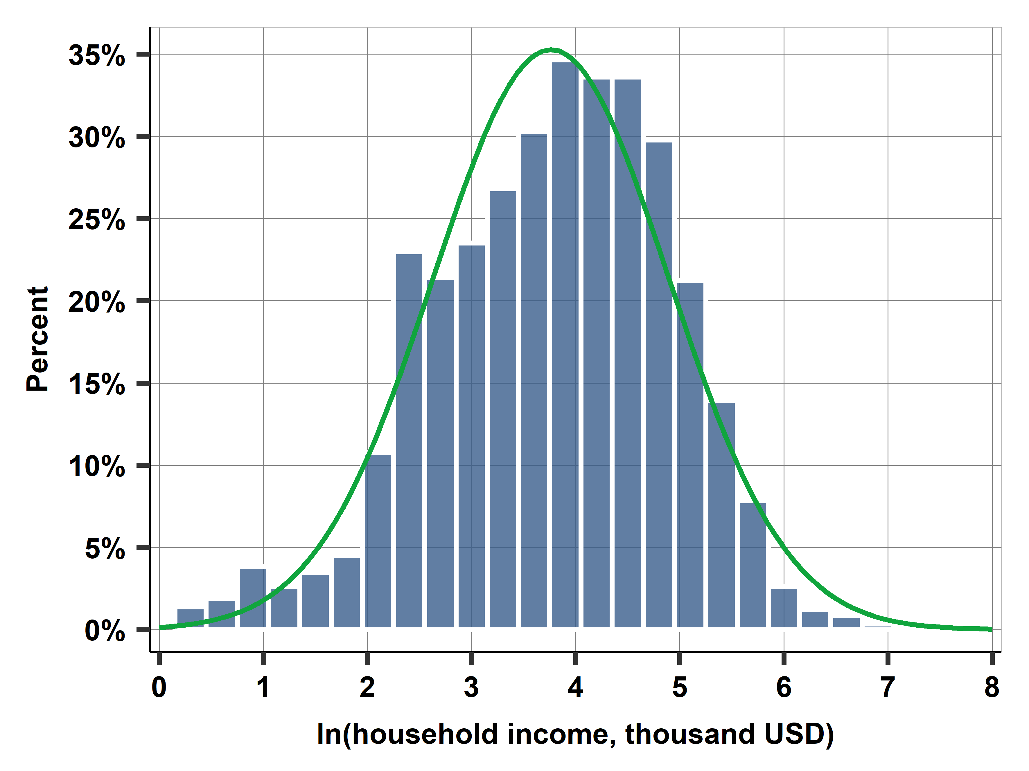
Ch03D Distributions of body height and income

Are the distributions of body heigh and family income well approximated by theoretical distributions? Answering these questions can help characterize their distributions and provide guidance for future analysis on how to use these variables.

In this very short case study, we examine survey data collected by the Health and Retirement Study in the U.S.A. in 2014 (height-income-distributions dataset). We show that the height of women aged 55-60 can be described by the normal distribution, whereas the income of their households is reasonably well characterized by the lognormal distribution.

Code: Stata or R or Python or ALL. Data: height-income-distributions. Graphs: .png or .eps

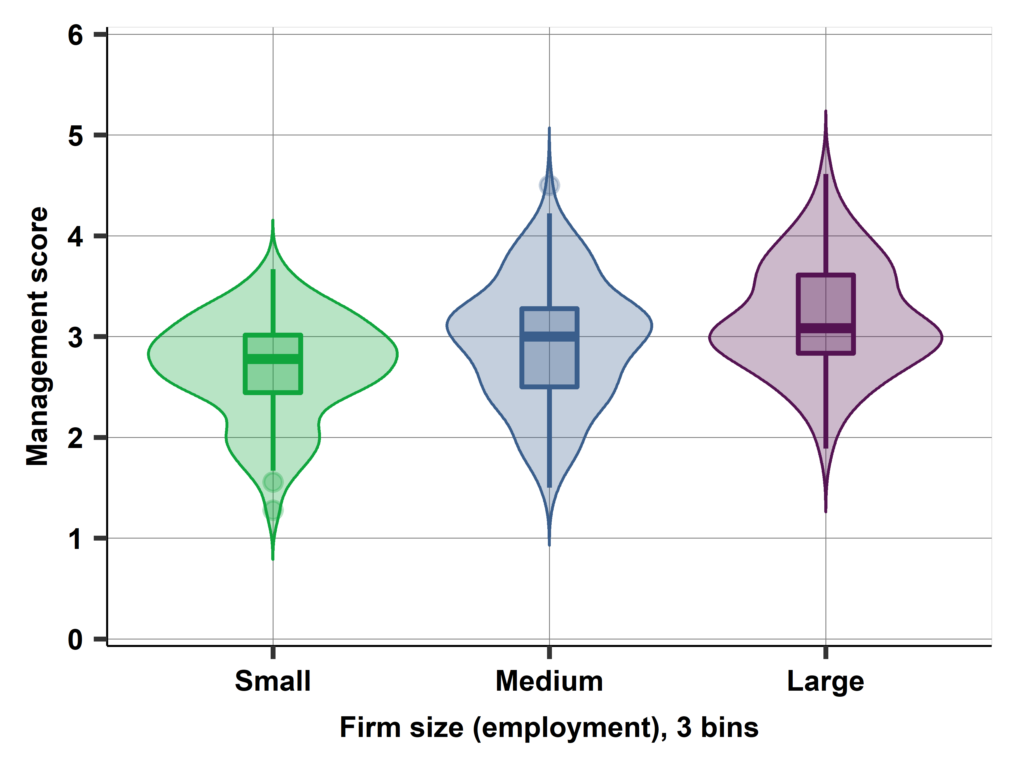
Ch04A Management quality and firm size: describing patterns of association

Are larger companies better managed? We want to explore the association between management quality and firm size in a particular country (Mexico). To answer this question we need to define the y and x variables in this comparison. In particular, we need to assess how the variables in the dataset correspond to the abstract concepts of management quality and firm size.

This case study uses the Mexican subsample of the World Management Survey dataset (wms-management-survey) from 2013. It illustrates how we can measure latent variables by proxy variables in the data and uncover patterns of association betewen those variables. It also illustrates the concepts of conditional probability, conditional distribution, and joint distribution. The case study introduces informative ways to visualize various aspects of patterns of association, such as the stacked bar chart, the scatterplot, the bin scatter, and comparing box plots and violin plots. We have introduced the data used here in case study 1C.

Code: Stata or R or Python or ALL. Data: wms-management-survey. Graphs: .png or .eps

CH05A What likelihood of loss to expect on a stock portfolio?

Can we find out the future likelihood of a large loss on a stock portfolio based on data from the past? We choose the S&P 500 stock market index as our investment portfolio, and we defining a large loss as an at least 5% drop in returns from one day to another. We can easily calculate the proportion of such days in the data, but we are interested in future losses not past ones. To answer our question we need to make generalizations from our data. Such generalizations are bound to bring uncertainty, and we would like to quantify that uncertainty, too.

This case study uses the sp500 dataset that covers day-to-day returns on the S&P 500 stock market index for 11 years to illustrate how we can generalize an estimated statistic from a particular dataset to the population, or general pattern, it represents, and beyond, to the general pattern we are interested in. The case study illustrates the concept of repeated samples. It shows how to estimate the standard error by bootstrap or using a formula, and how to construct and interpret a confidence interval. It also illustrates how to think about external validity. Case study 6B will use the same data to answer a related, but slightly different question.

Code: Stata or R or Python or ALL. Data: sp500. Graphs: .png or .eps

CH06A Comparing online and offline prices: testing the difference

Do online and offline prices of the same products tend to be the same? Answering this question can help make better purchase choices, understand the business practices of retailers, and it can inform whether we can use online data in approximating offline prices for policy analysis.

This case study uses the billion-prices dataset. We examine online and offline prices of retail products in the U.S. in 2015-16. The case study illustrates how to translate a more abstract question into an inquiry about a statistic (here the average difference). It shows how to formulate a null hypothesis and an alternative hypothesis and how to carry out a hypothesis test in two ways, by calculating the t-statistic and comparing it to an appropriate critival value, or, alternatively, by using the p-value. The case study also illustrates the perils of testing multiple hypotheses and p-hacking. We have introduced the data used here in case study 1B.

Code: Stata or R or Python or ALL. Data: billion-prices. Graphs: .png or .eps {:target=”_blank”}

CH06B Testing the likelihood of loss on a stock portfolio

Will our investment portfolio suffer a large loss with a higher chance than what we can accept? When we want to know what’s the likelihood of large future losses on our portfolio, we can use the confidence interval to quantify the uncertainty from estimating it from data on past returns. But we can ask a more pointed question, too: whether our stock portfolio is will suffer large future losses more often than we can accept. To answer that question we need a different procedure: testing a hypothesis.

This case study uses the sp500 dataset that covers day-to-day returns for 11 years to illustrate how we can test whether a likelihood is greater or less than a specified value. It illustrates testing proportions and how to formulate and carry out a one-sided hypothesis test. The case study is a continuation of case study 5A, using the same data.

Code: Stata or R or Python or ALL. Data: sp500. Graphs: .png or .eps